Data Science: Cental Limit Theorem

TLDR:

The Central Limit Theorem captures the following phenomenon:

Take any distribution! (say a distribution of number of passes in a football match)
Start taking n samples from that distribution (say n = 5) multiple times [say m = 1000] times.
Take mean of each sample set (so we would have m = 1000 means)
The distribution of means would be (more or less) normally distributed . (You will get that famous bell curve if you plot the means on x-axis and their frequency on y-axis.)
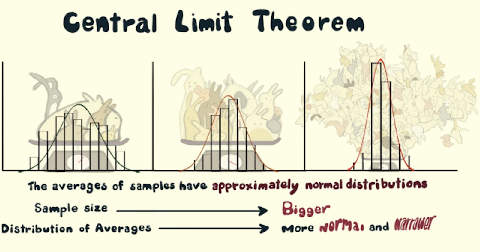
increase n to get a smaller standard deviation and increase m and to get a better approximation to normal distribution.

But why should I care?

Are you unable to load the whole data for processing? No problem, take out multiple samples from the data and use the central limit theorem to estimate the data parameters like mean, standard deviation, sum etc.
It can save you resources in terms of time and money. Because now we can work on samples significantly smaller than the population and draw inferences for entire population!
Does a certain sample belong to a certain population (or a data set)? Let's check that using the sample mean, population mean, sample standard deviation and population standard deviation.

Definition

Given a dataset with unknown distribution (it could be uniform, binomial or completely random), the sample means will approximate the normal distribution.

Explanation

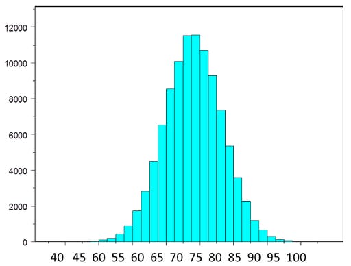
If we take any dataset or a population and we start taking samples from the population. Let's say we take 10 samples and take the mean of those samples. And we keep on doing this, a few number of times, say 1000 times. After doing this we get 1000 means and when we plot it, we get a distribution called a sampling distribution of sample means.

This sampling distribution (more or less) follows a normal distribution! This is the Central Limit theorem. A normal distribution has a number of properties which are useful for analysis.

Fig.1 Sampling distribution of sample means (following a normal distribution)

Properties of a normal distribution:

The mean, mode and median are all equal.
68% of the data falls within one standard deviation of the mean.
95% of the data falls within two standard deviations of the mean.
The curve curve is symmetric at the center (i.e. around the mean, μ).

Moreover, the mean of the sampling distribution of sample means is equal to the population mean. If μ is the population mean and μ_X̅ is the mean of the sample means then:

Fig.2 population mean = sample mean

And the standard deviation of the population(σ) has the following relation to the standard deviation sampling distribution (σ_X̅):

If σ is the standard deviation of population and σ_X̅ is the standard deviation of sample means, and n is the sample size, then we have

Fig.3 Relation between population standard deviation and sampling distribution standard deviation

Intuition

Since we are taking multiple samples from the population, the means would be equal (or close) to the actual population mean more often than not. Hence, we can expect a peak (mode) in the sampling distribution of sample means equal to the actual population mean.

Multiple random samples and their means would lie around the actual population mean. Hence, we can assume 50% of the means would be greater than the population mean and 50% would be less than that (median)

If we increase the sample size (from 10 to 20 to 30), more and more of the sample means would fall closer to the population mean. Hence the average(mean) of those means should be more or less similar to the population mean.

Consider The extreme case where the sample size is equal to the population size. So, for each sample, the mean would be same as the population mean. This is the narrowest distribution (standard deviation of sample means, here is 0)

Hence, as we increase the sample size (from 10 to 20 to 30) the standard deviation would tend to decrease (because the spread in the sampling distribution would be limited and more of the sample means would be focused towards population mean). This phenomenon is captured in the formula in "Fig. 3" where the standard deviation of the sample distribution is inversely proportional to the square root of sample size.

If we take more and more samples (from 1,000 to 5,000 to 10,000), then the sampling distribution would be a more smoother curve, because more of the samples would behave according to the central limit theorem and the pattern would be cleaner.

"Talk is Cheap, show me the code!" - Linus Torvalds

So lets simulate the central limit theorem via code:

Some Imports:

import random
from typing import List
import matplotlib.pyplot as plt
import matplotlib
import statistics
import pandas as pd
import math

Create a population using random.randint(). You can try different distributions to generate data. The following code generates a (sort of) monotonically decreasing distribution:

def create_population(sample_size: int) -> List[int]:
    """Generate a population of sample_size

    Args:
        sample_size (int): The size of the population

    Returns:
        List[int]: a list of randomly generated integers
    """
    population = []
    for _ in range(sample_size):
        random_number = (random.randint(0, random.randint(1, 1000)))
        population.append(random_number)
    return population

Create samples and take their mean sample_count number of times:

def generate_sample_mean_list(population: List[int],
                              sample_size: int,
                              sample_count: int) -> List[int]:
    """From the population generate samples of sample_size, sample_count times

    Args:
        population (List[int]): List of random numbers
        sample_size (int): Number of elements in each sample
        sample_count (int): Number of sample means in sample_mean_list

    Returns:
        List[int]: a list of sample means
    """
    sample_mean_list = []
    for _ in range(sample_count):
        sample = random.sample(population, sample_size)
        sample_mean = statistics.mean(sample)
        sample_mean_list.append(sample_mean)
    return sample_mean_list

Function to plot the distribution of data along with some labels

def plot_hist(data: List[int],
              ax: matplotlib.axes.Axes,
              xlabel: str,
              ylabel: str,
              title: str,
              texts: List[str]) -> None:
    """Plot a histogram with labels and additional texts

    Args:
        data (List[int]): the list of data points to be plotted
        ax (matplotlib.axes.Axes): Axes object for text plotting
        xlabel (str): label on x axis
        ylabel (str): label on y axis
        title (str): title of the plot
        texts (List[str]): Additional texts to be plotted
    """
    plt.hist(data, 100)
    plt.xlabel(xlabel)
    plt.ylabel(ylabel)
    plt.title(title)

    i = 0.0
    for text in texts:
        plt.text(0.8,
                 0.8 - i,
                 text,
                 horizontalalignment="center",
                 verticalalignment="center",
                 transform=ax.transAxes)
        i += 0.05
    plt.grid(True)
    plt.show()

Main function to run the code:

def main(plot=True):
    """Driver Function

    Args:
        plot (bool, optional): Decide whether to plot or not. Defaults to True.
    """
    fig, ax = plt.subplots()
    population_size = int(1E5)
    population = create_population(population_size)
    if plot:
        plot_hist(population,
                  ax,
                  "Value",
                  "Frequency",
                  "Histogram of Population of Random Numbers",
                  [f"population_size={population_size}"])

    population_mean = statistics.mean(population)
    population_stdev = statistics.stdev(population)

    sample_size_list = [50, 500]
    sample_count_list = [500, 5000]

    records = []
    for sample_size in sample_size_list:
        for sample_count in sample_count_list:
            sample_mean_list = generate_sample_mean_list(
                population, sample_size, sample_count)

            # also called as mean of sample distribution of sample means
            mean_of_sample_means = round(statistics.mean(sample_mean_list), 2)

            # also called standard dev of sample distribution of sample means
            std_error = round(statistics.stdev(sample_mean_list), 2)
            if plot:
                plot_hist(sample_mean_list,
                          ax,
                          "Mean Value",
                          "Frequency",
                          "Sampling Distribution of Sample Means",
                          [
                              f"sample_count={sample_count}",
                              f"sample_size={sample_size}",
                              f"mean_of_sample_means={mean_of_sample_means}",
                              f"std_error={std_error}"])

            record = {
                "sample_size": sample_size,
                "sample_count": sample_count,
                "population_mean": population_mean,
                "sample_mean": mean_of_sample_means,
                "population_stdev": population_stdev,
                "population_stdev_using_formula": std_error*math.sqrt(sample_size),
                "sample_stdev": std_error,
            }

            records.append(record)

    df = pd.DataFrame(records)
    print(df)


if __name__ == "__main__":
    main(plot=True)

You can find the whole code here on Github

Hemal Mamtora's Blog